Format as Table

Tables have many benefits in Excel: default styling, filters, and the ability to easily insert rows or columns. When you create a table, you'll need to specify a header row. Table headers help screen reader users track where they are when navigating through the cells of your table.

To format your data as a table with column headers:

1. Highlight the rows and columns in your sheet that you would like to format as a table.
2. Navigate to the Home tab in the ribbon.
3. Select the Format as Table dropdown.
4. Choose a default Table Style or create a New Table Style.
   
   Pro Tip: Go with a Table Style that uses banded rows (i.e., alternating background colors for each row) so that your rows are more visually distinct. Always make sure your text has sufficient color contrast against the table's background colors. 
   

   

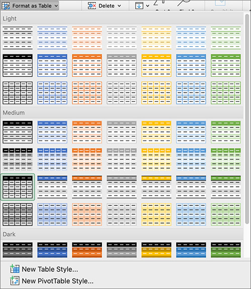
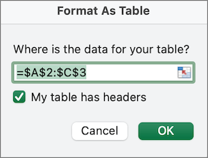
5. Select the checkbox My table has headers and press OK.
   

   

If your table also has a row header, then select the checkbox First Column under the Table tab in the ribbon.

Set a Table Name

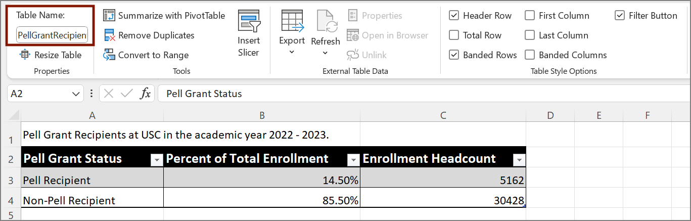
After you create a table in Excel, it will have a default Table Name (e.g., Table1) within the Table Design tab of the ribbon on Windows, or within the Table tab on Mac. Use upper camel case (i.e., capitalize the first letter of each word and leave no spaces between words) to give a unique name to your table. The Table Name provides screen reader users with context about what table they are interacting with. 

Example: 

Define Names for Table Headers

In order for NVDA and JAWS screen readers on Windows to read out table headers properly, the table headers must be marked up with a Title Region using the Define Name function. The following conventions will tell a screen reader what type of headers are available:

TitleRegion: your table has both column and row headers.

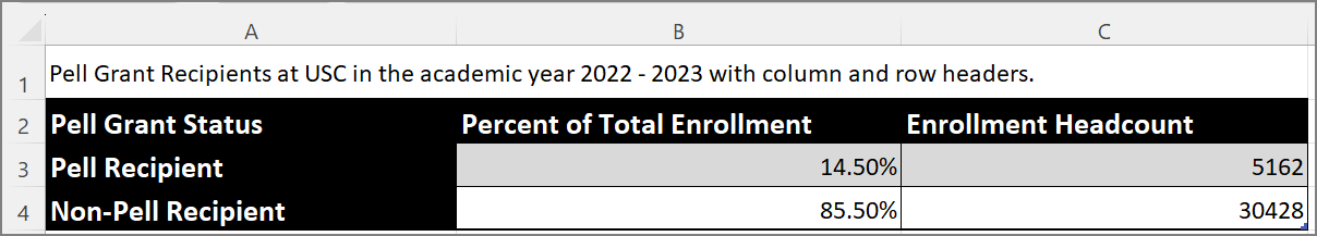
ColumnTitleRegion: your table has only column headers, which are in the top row of your table.

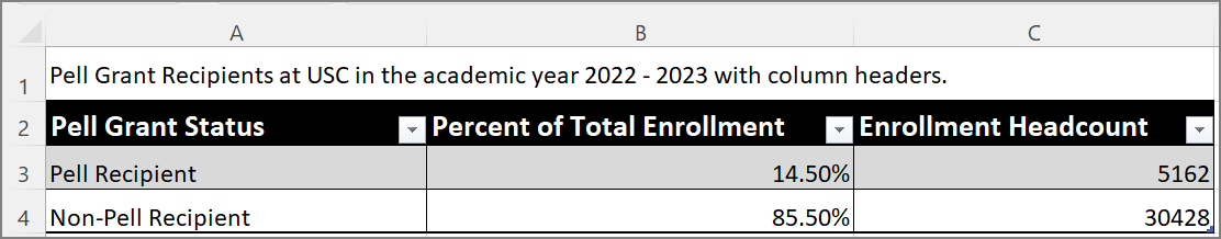
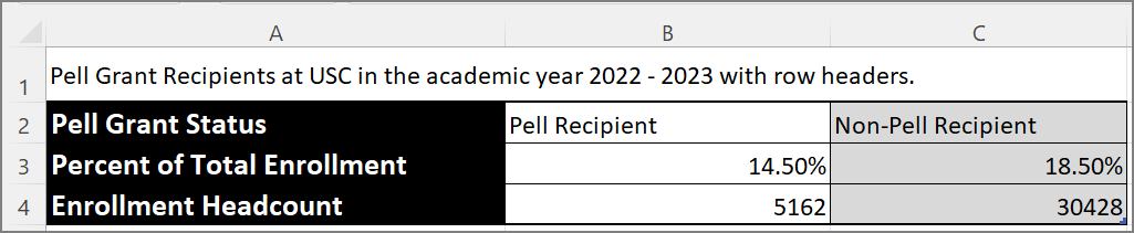
RowTitleRegion: your table has only row headers, which are in the first column of your table.

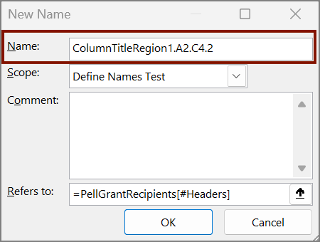
It's a best practice to only have one table per sheet; however, if you have multiple tables on one sheet, the following naming convention will tell the screen reader where to apply your Title Region: 

[Type of Header][Table Number].[Top Left Cell Address].[Bottom Right Cell Address].[Worksheet Number]

Example: TitleRegion1.A2.C4.1

Steps for Defining Names

1. Highlight the table headers you plan to define a Title Region for.
2. Navigate to the Formulas tab in the ribbon.
3. Open the Define Name dropdown and select Define Name.
4. Following the conventions provided above, fill in a unique Name.
   

   

5. Select your current sheet for the scope and press OK.

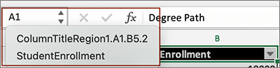
While the process to define names may feel cumbersome, it can make a dramatic difference for how understandable your data is to a screen reader user. Not only does this allow screen reader users to hear row and/or column headers as they navigate through the data cells, but it also allows them to more easily navigate to the tables using the Name Box.